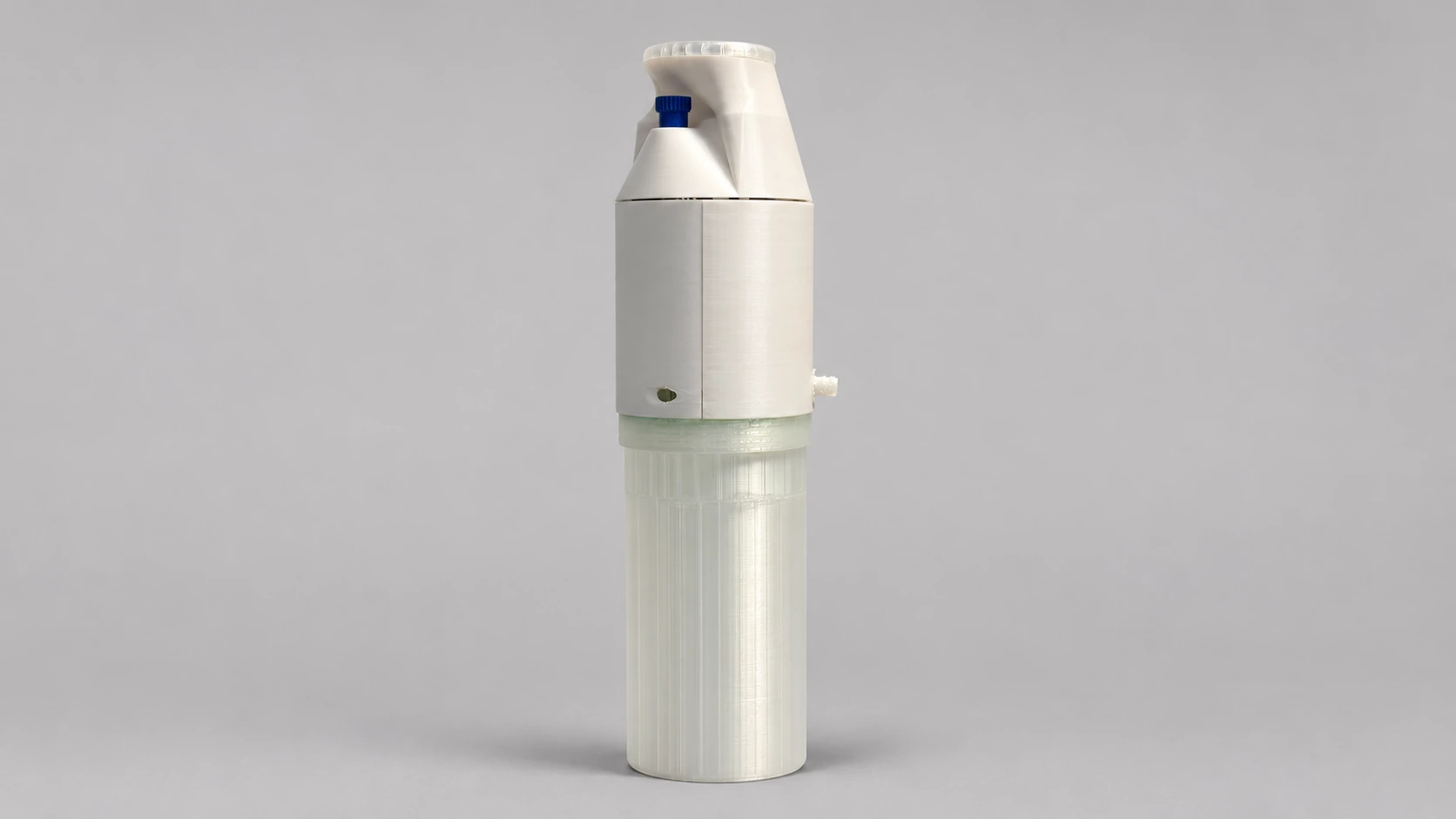
Portable cocktail mixer
Prototyping
I design electronics
and build useful things.
Flynn Studio brings together my independent projects and collaborations. I start with everyday questions and real needs, using engineering to turn ideas into useful things.
During a visit to Jackson Ranch, I was warmly welcomed by its owner. I offered to help redesign the ranch’s existing website—a way to give something back through my work.
Website redesign · In progress
View original websiteI’m Flynn Mi, an electrical engineer who loves life. The experiences I’ve had have shaped how I see the world, and I’m grateful for the people who have helped and inspired me along the way.
My work focuses on electronics, embedded systems, and product prototyping. I enjoy turning an idea into something that works, learning through building, testing, and refining. Each iteration brings the problem into sharper focus, along with a better understanding of how the product can serve the person using it. That gradual movement from uncertainty to clarity is a challenge I find deeply rewarding.
Flynn Studio is where I put this curiosity into practice. It brings together my independent projects and collaborations across different fields, grounded in an engineering perspective. Through this work, I hope to keep growing and create things that bring a little ease, joy, and beauty to everyday life.
If you’d like to collaborate, share an idea, or simply say hello, I’d love to hear from you.
Brown University
Sc.M. · Electrical & Computer EngineeringJinan University
B.Eng. · Communication EngineeringFlynn Studio · Independent Practice
2026–PresentBrown CSSA · Vice President
2025–2026Digital integrated circuits · ENGN 1600
From multiplier architectures to physical implementation.
I compared multiplier architectures and array sizes to understand their area, timing and throughput trade-offs. The 50-point array sweep found nonnegative post-route setup slack across all five sizes at 833.33 MHz.
Overview
The study connects two scales of digital design: how a multiplier schedules arithmetic, and how a systolic array scales computation. The multiplier labs establish the RTL-to-layout workflow; the final project applies implementation analysis to a course-provided array framework.
My focus was to connect architectural choices with verifiable results: transaction rate, cell area, setup margin and workload-dependent throughput.
The final-project array RTL and testbench were supplied by the course. My work on that framework centers on verification, implementation exploration and analysis.
Four implementations of a 32-bit unsigned multiplier exposed the cost of parallelism and resource reuse. Design Compiler mapped each RTL description to standard cells; the resulting structures differed substantially in area, critical-path depth and transaction rate.
Multiplier synthesis baseline NangateOpenCellLibrary / FreePDK45 · typical corner · 2.00 ns clock target.
| Architecture | Implementation trade-off |
|---|---|
| V0 Operator-inferred | A registered a * b baseline lets synthesis choose the arithmetic implementation. |
| V1 Combinational shift-add | Partial products are combined within one cycle, exposing a long combinational path. |
| V2 Iterative shift-add | A reused adder reduces hardware; a non-overlapping operation needs one load and 32 update cycles. |
| V3 Pipelined multiplier | Stage registers support a new input each cycle, at the cost of additional state and clock load. |
The iterative datapath advances one bit per cycle. Its initiation interval is at least 33 cycles for W = 32; the pipelined design can accept a new transaction every cycle. Comparing clock frequency alone would miss this architectural difference.
else if (v[W-1:0] != 0) begin
    if (b_reg[0])
        p_reg <= p_reg + a_reg;

    a_reg <= a_reg << 1;
    b_reg <= b_reg >> 1;
end
Datapath update only; reset, input loading and valid control omitted.
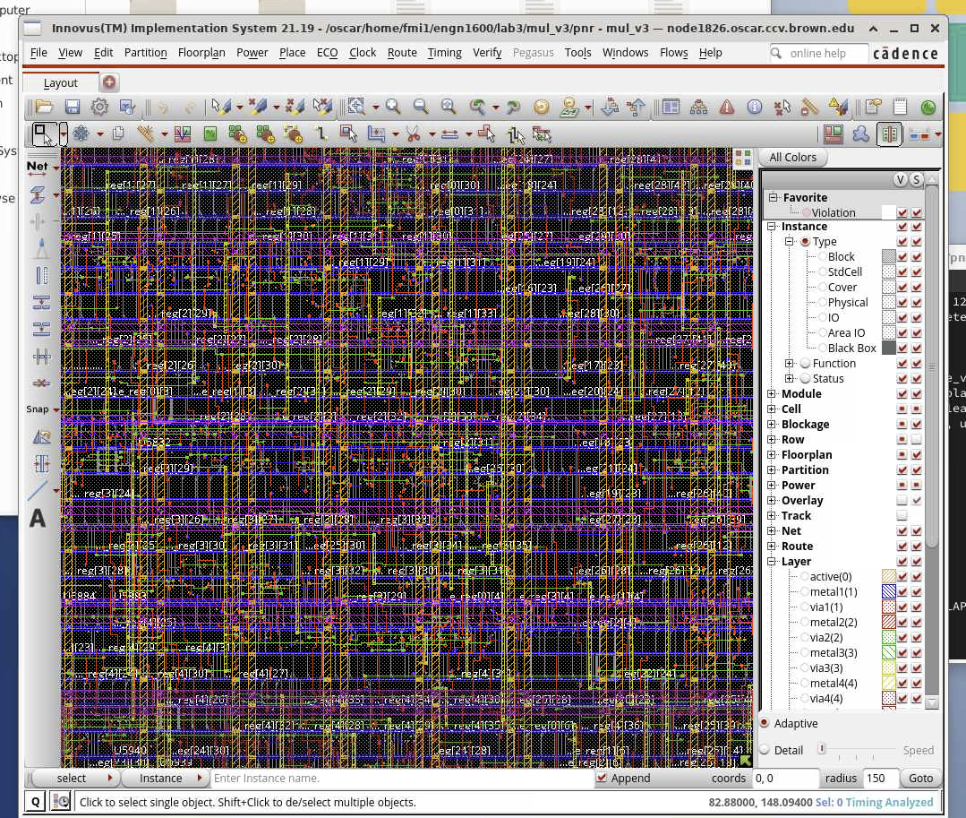
Cadence Innovus carried the synthesized multiplier through placement and routing. The layout makes the physical cost of pipeline registers, interconnect and clock distribution tangible. Post-route timing then tests the design against its clock constraint.
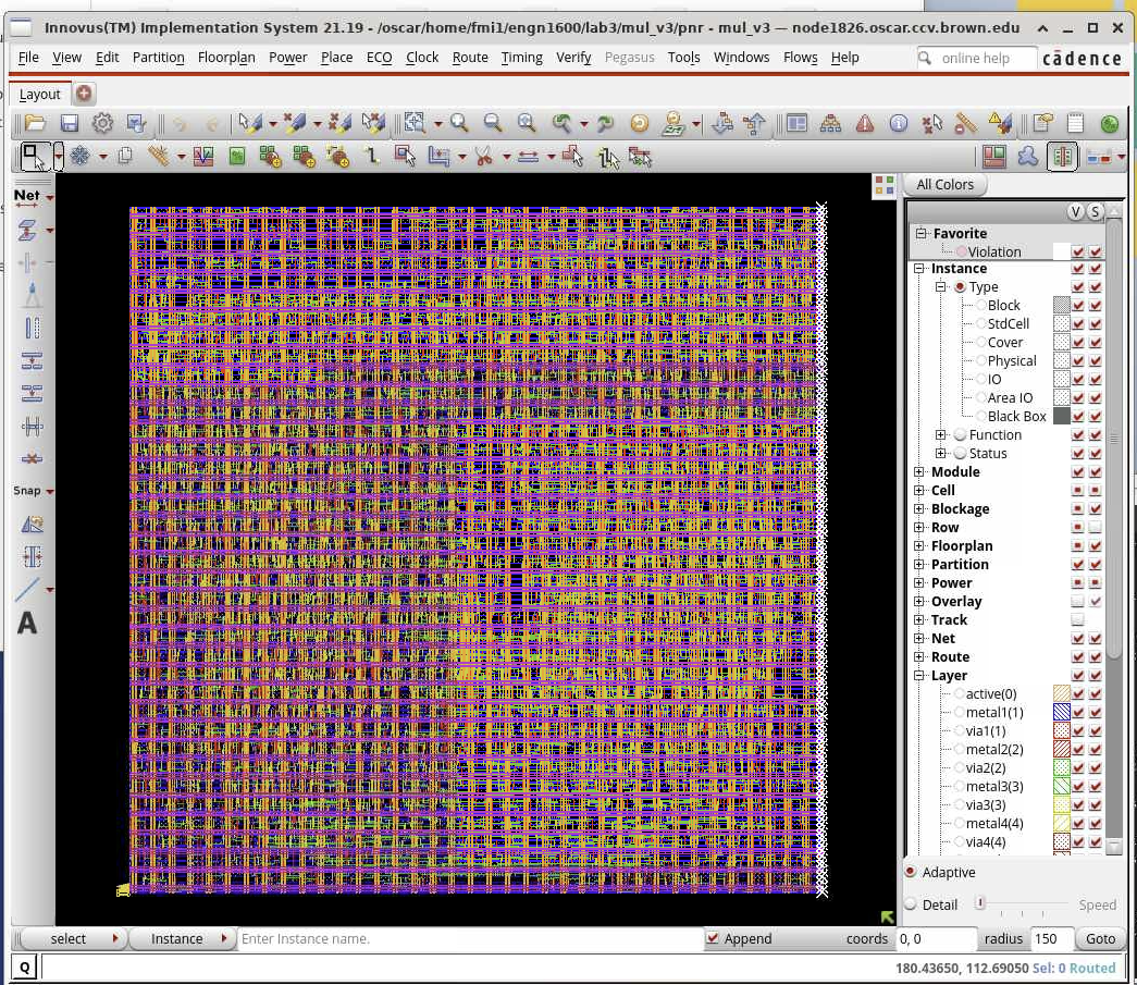
A timing path, after routing
+0.308 ns
Reported setup slack · 2.00 ns clock
The reported path meets the setup constraint. Slack measures the margin between required and arrival time; the arrival timestamp alone is not the path delay.
Lab 3 · design_pnr_timing.rpt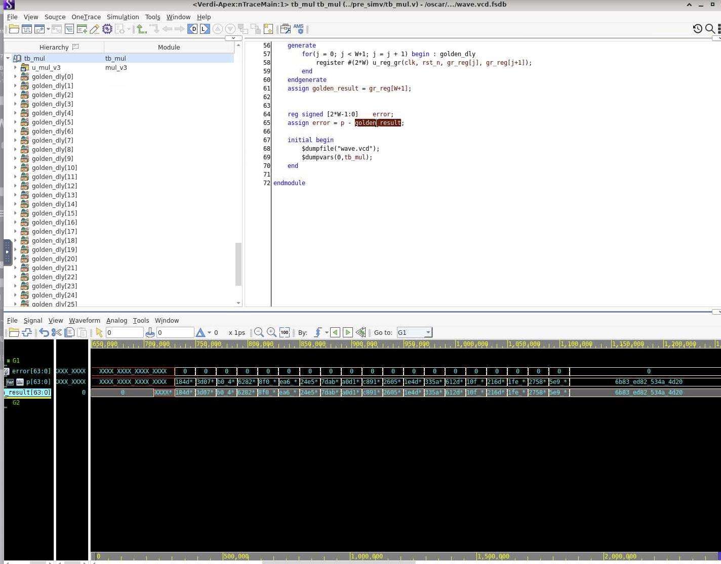
The power experiment used VCS waveform activity, converted from VCD to SAIF, with the routed netlist and SPEF parasitics in PrimeTime. It examined internal, net-switching and leakage power. The retained stimulus schedules and measurement windows differ, so these runs support exploratory power analysis rather than a normalized power ranking.
I checked 4×4, 6×6, 8×8, 12×12 and 16×16 configurations against reference matrix results. Staggered operands travel between neighboring processing elements, where multiply-accumulate operations build each output.
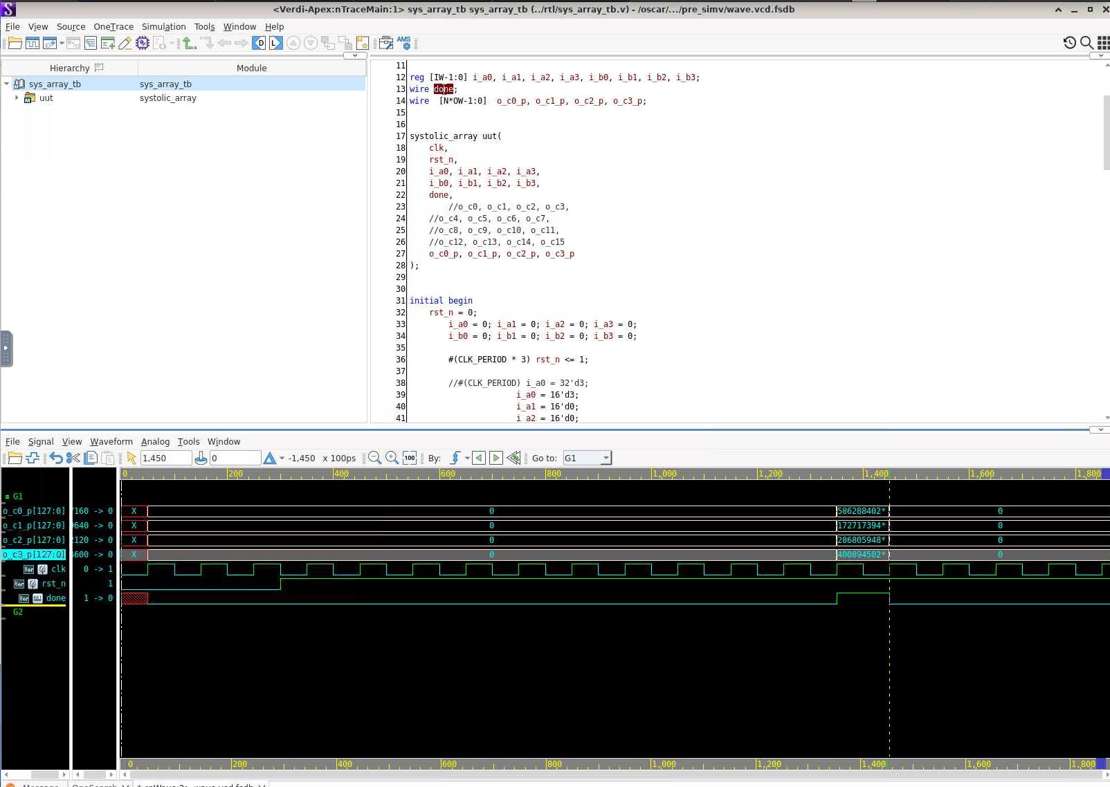
The 4×4 case performs 64 MACs over ten compute cycles in the ideal schedule. Verification checks both when the output is valid and whether its values match the reference.
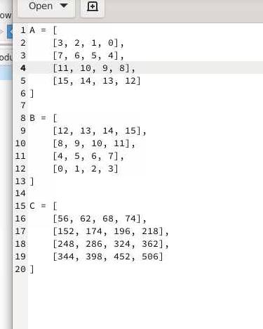
done = 1| 56 | 62 | 68 | 74 |
| 152 | 174 | 196 | 218 |
| 248 | 286 | 324 | 362 |
| 344 | 398 | 452 | 506 |
The waveform displays packed buses. I checked them at the asserted done signal and compared the matrix results with the reference data. The report records the matching bottom-right element, C[3][3] = 506.
The matrix shown here is transcribed from the report’s expected result; it is not a direct numeric readout of the packed waveform.
Each array size was evaluated at ten target periods, from 2.6 ns to 0.8 ns. The 50-point sweep records synthesis and post-route area alongside setup slack. Area grows approximately with N², while tighter clock targets change the implementation cost and feasibility.
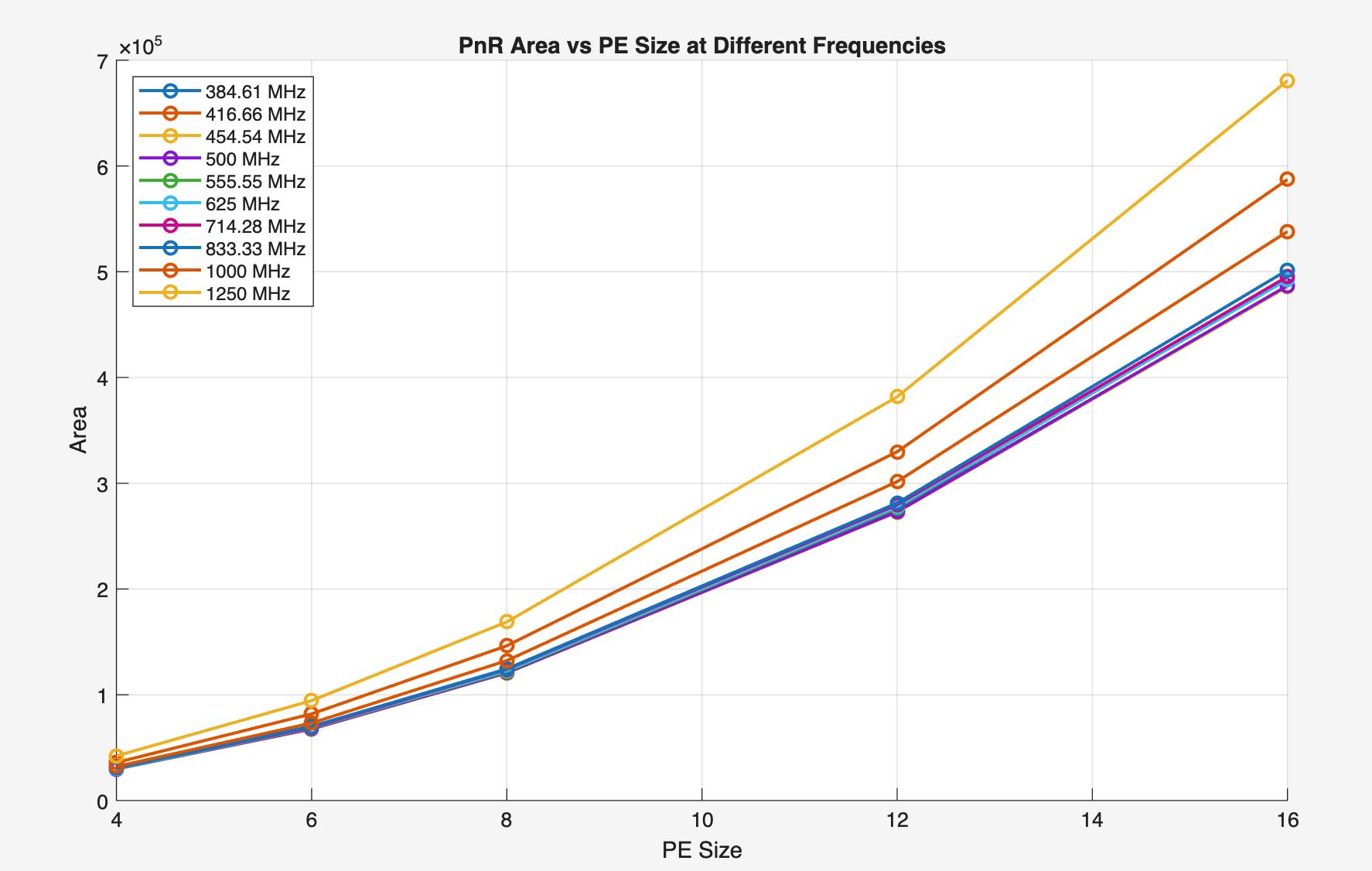
All five arrays have nonnegative reported post-route setup slack at 833.33 MHz. At 1 GHz, only the 4×4, 6×6 and 8×8 runs meet that criterion; all five miss it at 1.25 GHz.
These are sampled timing results, not exact maximum operating frequencies or full sign-off.
| Array | 833.33MHz | 1,000MHz | 1,250MHz |
|---|---|---|---|
| 4×4 | +0.019 | +0.014 | −0.102 |
| 6×6 | +0.014 | +0.009 | −0.123 |
| 8×8 | +0.019 | +0.010 | −0.119 |
| 12×12 | +0.005 | −0.012 | −0.119 |
| 16×16 | +0.013 | −0.027 | −0.142 |
Negative slack misses the setup constraint. Values transcribed from the array implementation summaries.
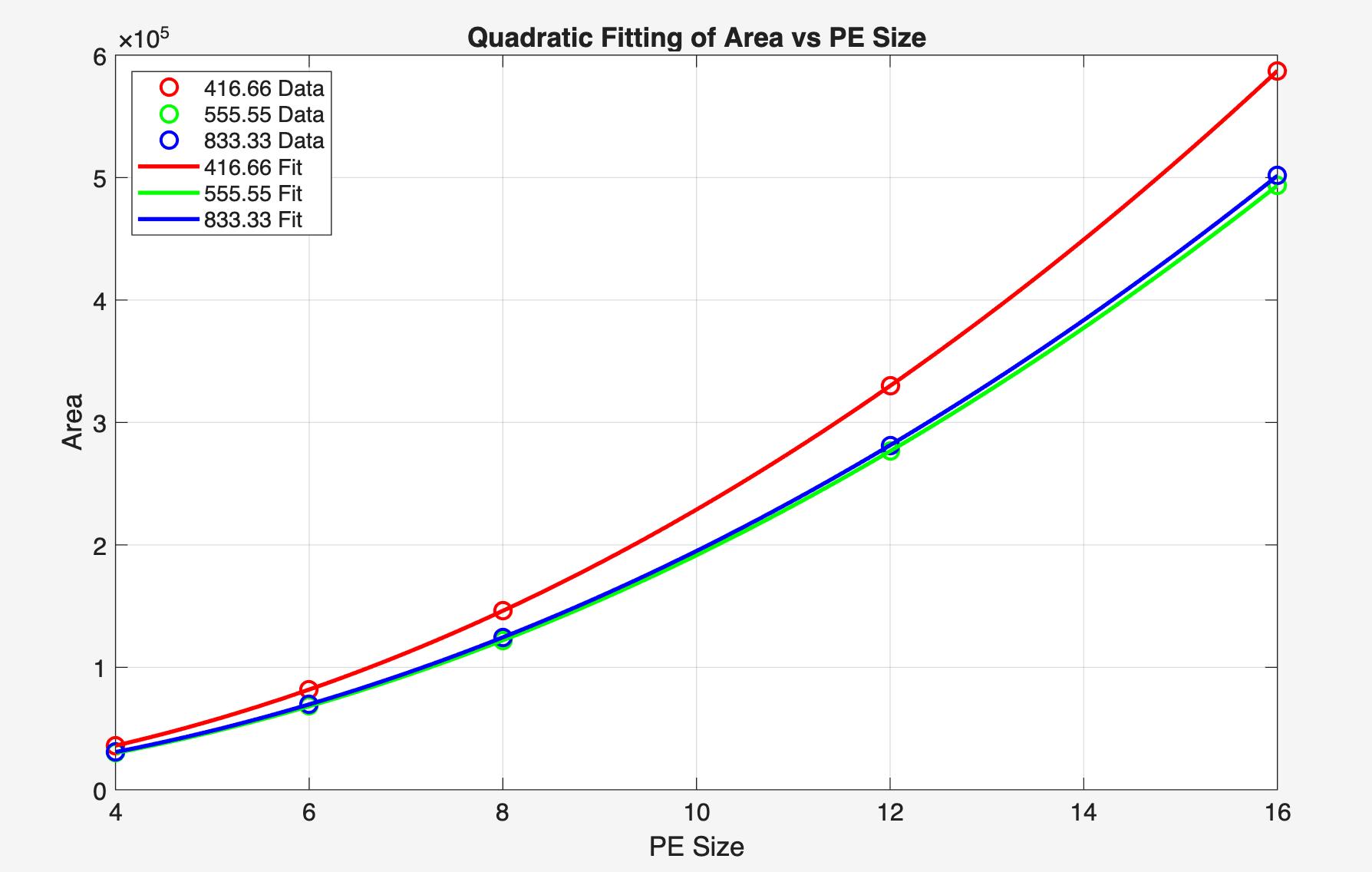
MATLAB fits of A(N) = aN² + bN + c capture the sampled area trend. The fit supports design selection within the explored range; an unimplemented size remains an estimate.
This finite-tile model counts a multiply and an add as two operations, including array fill and drain. At 500 MHz it gives 89.04 GOPS for N = 16, before memory, I/O and scheduling overhead. It is a compute model, not measured chip throughput.
Engineering conclusions
At 500 MHz, growing from 4×4 to 16×16 increases reported cell area by 16.3×, while ideal finite-tile throughput rises by 13.9×. The area cost grows faster than useful throughput under this model.
| Array | Post-route cell area µm² | Modeled throughput GOPS |
|---|---|---|
| 4×4 | 29,857 | 6.40 |
| 8×8 | 120,711 | 23.27 |
| 16×16 | 486,862 | 89.04 |
Cell areas are rounded. Throughput uses 2N³ × f / (3N − 2), with each tile matched to array dimension N; memory, I/O and scheduling overhead are excluded.
For a 1 GHz target, only the sampled 4×4, 6×6 and 8×8 runs meet the reported setup constraint. This gives a practical selection order: filter by timing, then compare throughput against the area budget and workload assumptions.
Figures are extracted from my ENGN 1600 reports. Layout images show the Lab 3 multiplier; array results come from the final project. Timing values are reported EDA results; throughput values are analytical estimates.
3D photography · ENGN 2502 · 2024
From laser-line pixels to a colored point cloud.
I implemented the C++ image-processing and geometry routines behind a laser-scanning workflow: calibrating the scene, locating laser profiles and reconstructing them in a shared 3D coordinate system.
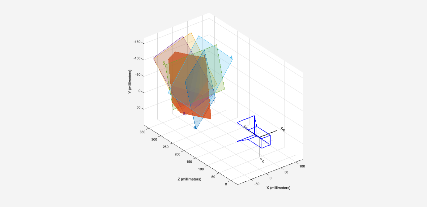
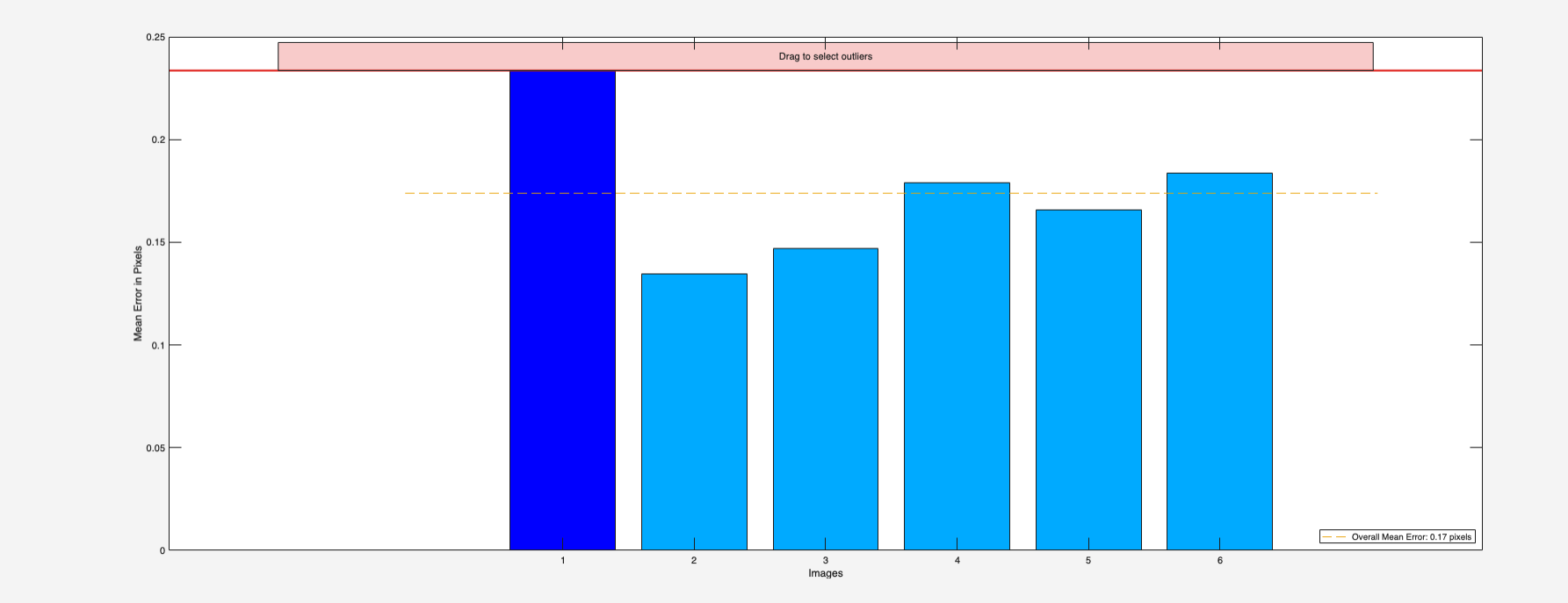
I implemented checkerboard reprojection: transform 3D points into the camera frame, apply perspective division and radial/tangential distortion, then map to pixels using the intrinsic matrix.
0.17 px
Mean reprojection error · Six-view MATLAB run
This measures image-plane fit. The later scanning dataset has a separate calibration.
For scanner geometry, I implemented SVD-based checkerboard pose estimation and laser-plane fitting, plus a least-squares solution for the turntable reference frame.
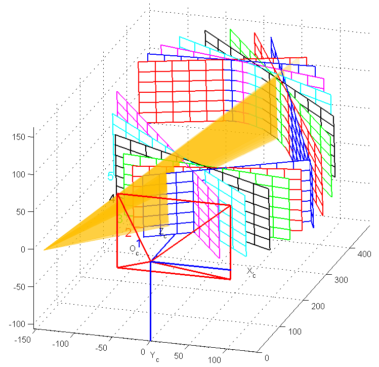
Pose: build a 2N × 9 homogeneous system, solve with SVD, recover scale and orthogonalize the rotation estimate. This pose routine ignores distortion; reprojection and triangulation handle it separately.
Plane: intersect detected rays with checkerboard planes, center the resulting 3D samples and extract the plane normal using SVD.
Turntable: solve for a center shared across rotated poses, then construct the turntable frame. One center coordinate is supplied in the vertical-checkerboard formulation.
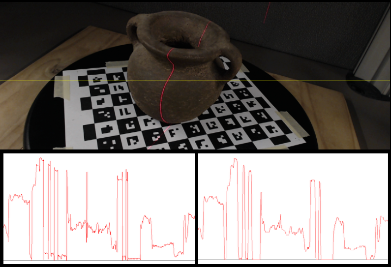
The detector progressed from single-image red-response extraction to laser-on/off differencing. I implemented the stages below to turn a bright stripe into image coordinates and associated colors.
| Stage | My implementation |
|---|---|
| Smooth | Separable convolution with the normalized [1, 4, 6, 4, 1] kernel. |
| Isolate | R − (G + B) / 2; later, ΔR − (ΔG + ΔB) / 2 from aligned on/off images. |
| Select | Restrict the search to a polygonal ROI and threshold the row-wise response. |
| Refine | Three-pixel intensity centroid for subpixel x; RGB sampled from the laser-off image. |
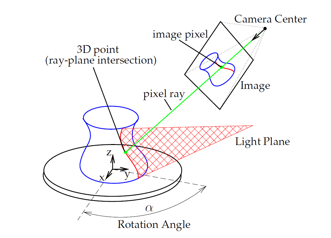
I mapped detected pixels through the inverse camera intrinsics to form rays, intersected them with the laser plane and transformed the points into the object frame. Undoing the turntable rotation aligns successive profiles.
My Assignment 3 routine iteratively compensates for lens distortion before the intersection.
When a ray is nearly parallel to the plane, nᵀr approaches zero and depth becomes sensitive to small errors. My routine skips these intersections.
double denominator =
    plane_normal.dot(u_norm);
if (std::abs(denominator) < 1e-6) {
    continue;
}

double lambda = -plane_d / denominator;
Vector3d X = lambda * u_norm;
worldPoints.push_back(X);
Ray normalization and inverse distortion precede this block.
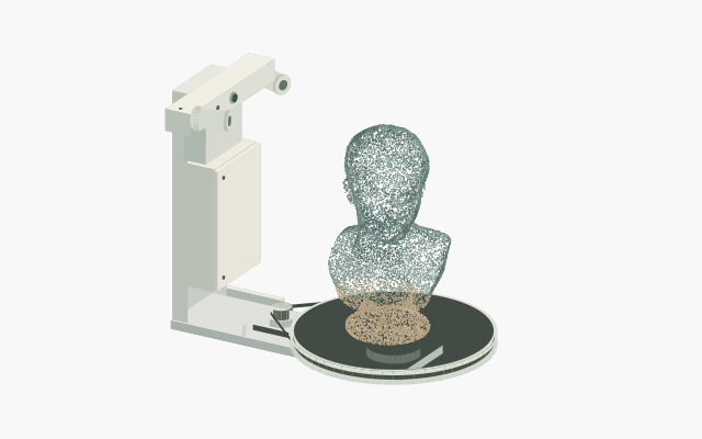
The reconstruction shown at the top recovers the statue and pedestal with sampled color. The application capture records both laser channels selected and a 4° per-frame setting.
The overall shape is recognizable. Separated scan profiles, background points and incomplete surface coverage remain visible.
Compare detections with the source images, inspect plane-fit residuals and compare individual profiles before merging. These checks would help separate extraction errors from geometric misalignment.
These are proposed diagnostic steps, not verified causes or completed improvements. No dimensional-accuracy measurement is claimed.
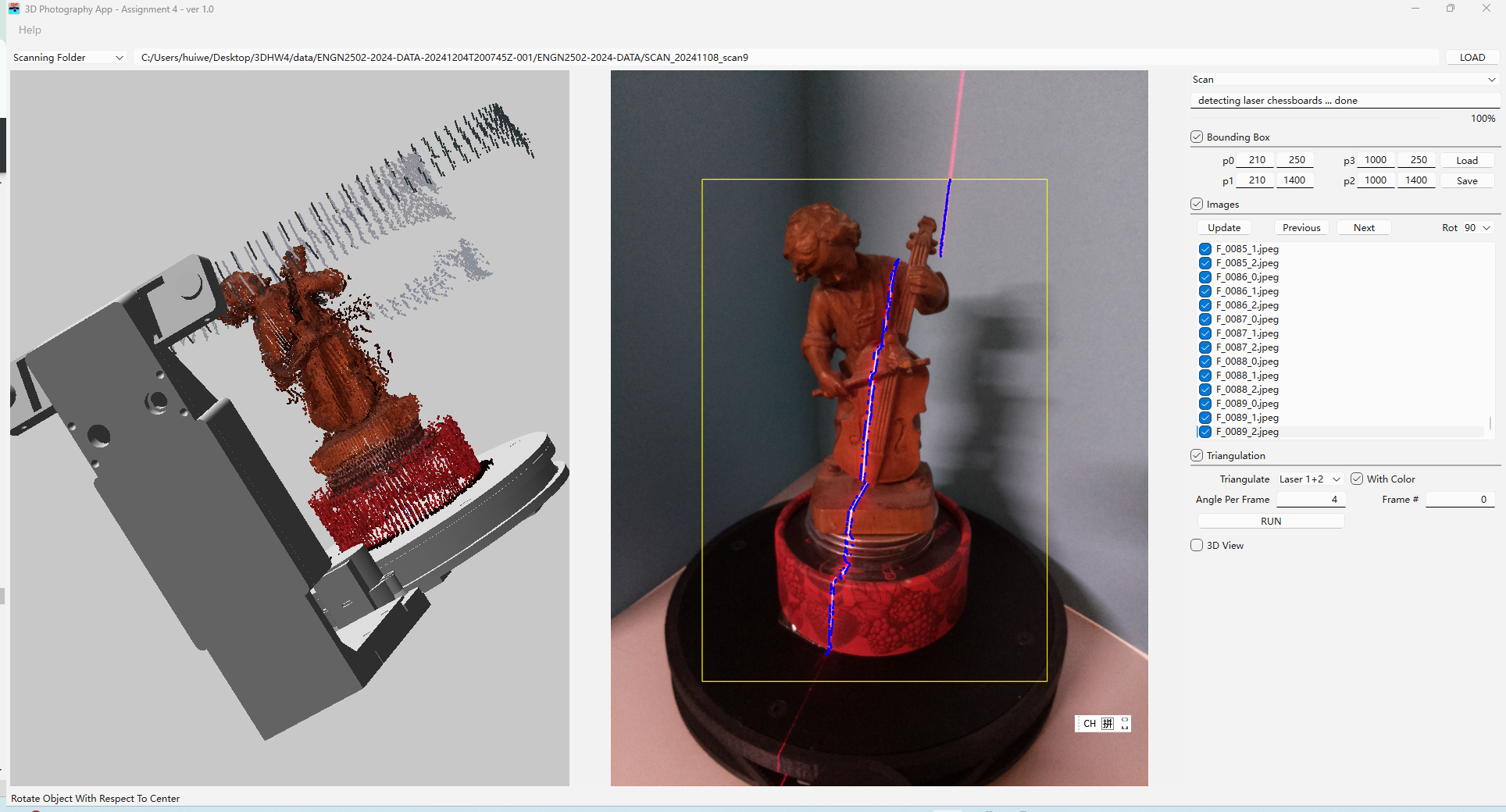
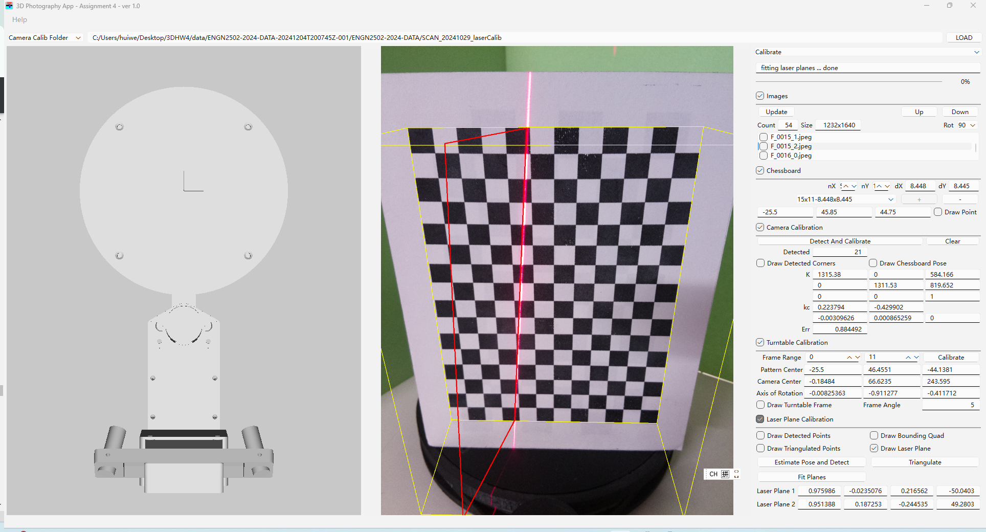
The scanner interface displays Err = 0.884492. Its metric definition has not been verified here, so it is kept separate from the six-view MATLAB mean of 0.17 px.
What this project demonstrates
I connected pixel-level detection with numerical estimation and 3D transforms in C++. The result is a working coursework reconstruction pipeline, with intermediate outputs that make both its behavior and limitations inspectable.
Implementation details are grounded in my submitted routines. My outputs and course references are labeled separately. Reference figures: Brown ENGN 2502, Fall 2024, Assignments 01–03, by Daniel Moreno, Peter Walecki and Gabriel Taubin. Course description ↗
Self-initiated product development
Guided mixing, from recipe to pour.
The product idea
Making a cocktail asks a beginner to coordinate a recipe, ingredient quantities and several tools. I proposed a handheld mixer that brings guidance and liquid intake into one device, while preserving the physical ritual of shaking and pouring.
I developed the concept and led a four-person team, owning the power system and mechanical design.
01 / Product strategy
Designed for home gatherings and people learning to mix drinks, the product keeps recipe guidance at the point of use. Its architecture follows the preparation sequence.
Choose a recipe with the rotary control.
Draw each ingredient into the cup, following the on-screen prompts.
Mix by hand within the handheld body.
Detach the cup and serve.
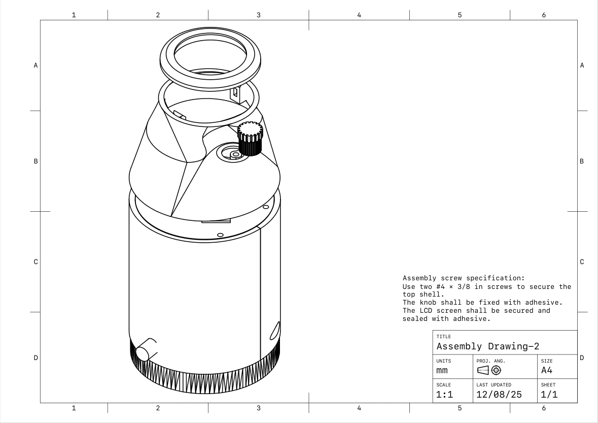
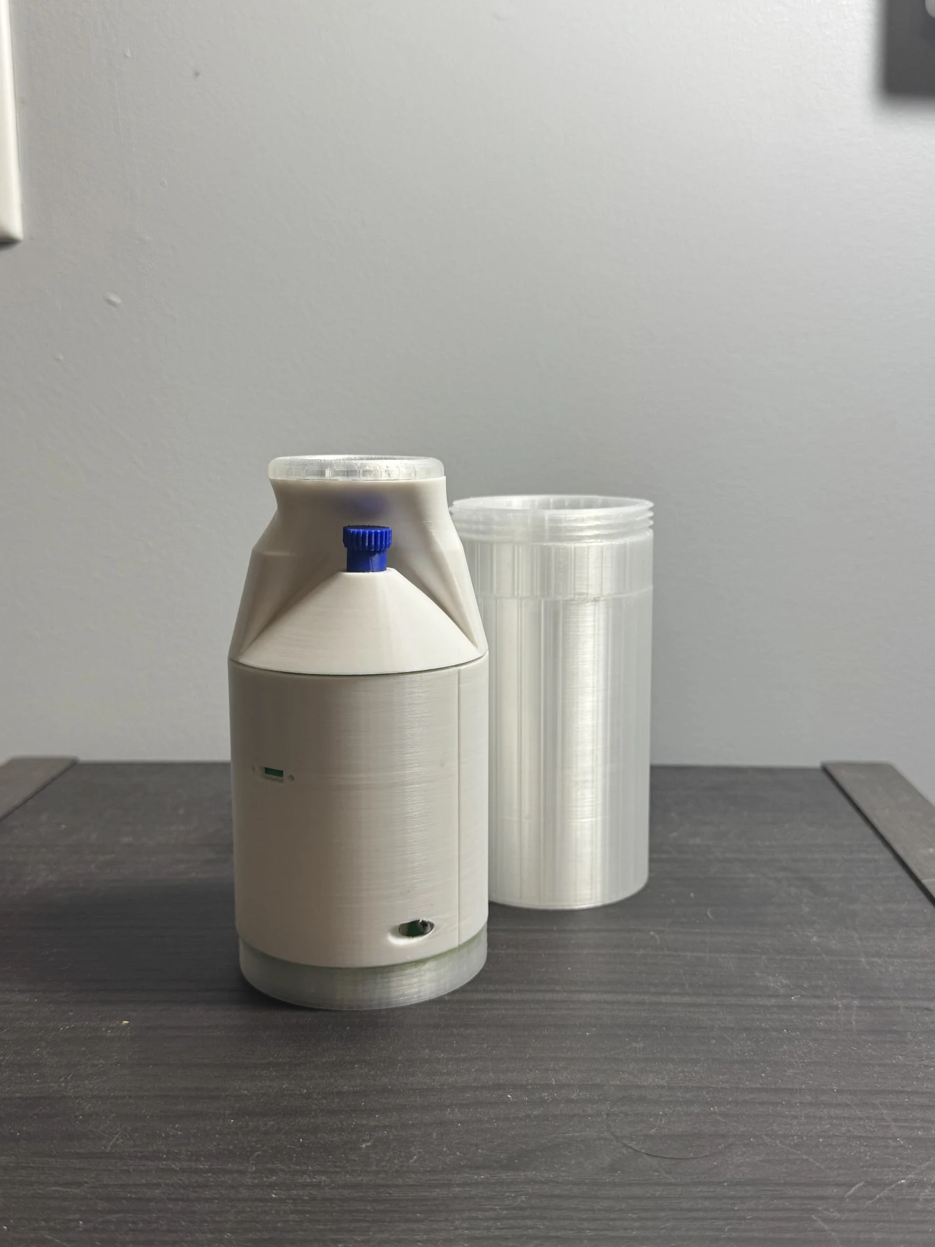
The display and knob guide preparation. The threaded cup handles serving. The split housing provides assembly access. Separating these interactions keeps routine use distinct from working on the internal hardware.
02 / Mechanical architecture
The handheld form sets the packaging envelope. Inside it, component locations, wiring space and fastening access determine how the product can be assembled and maintained.
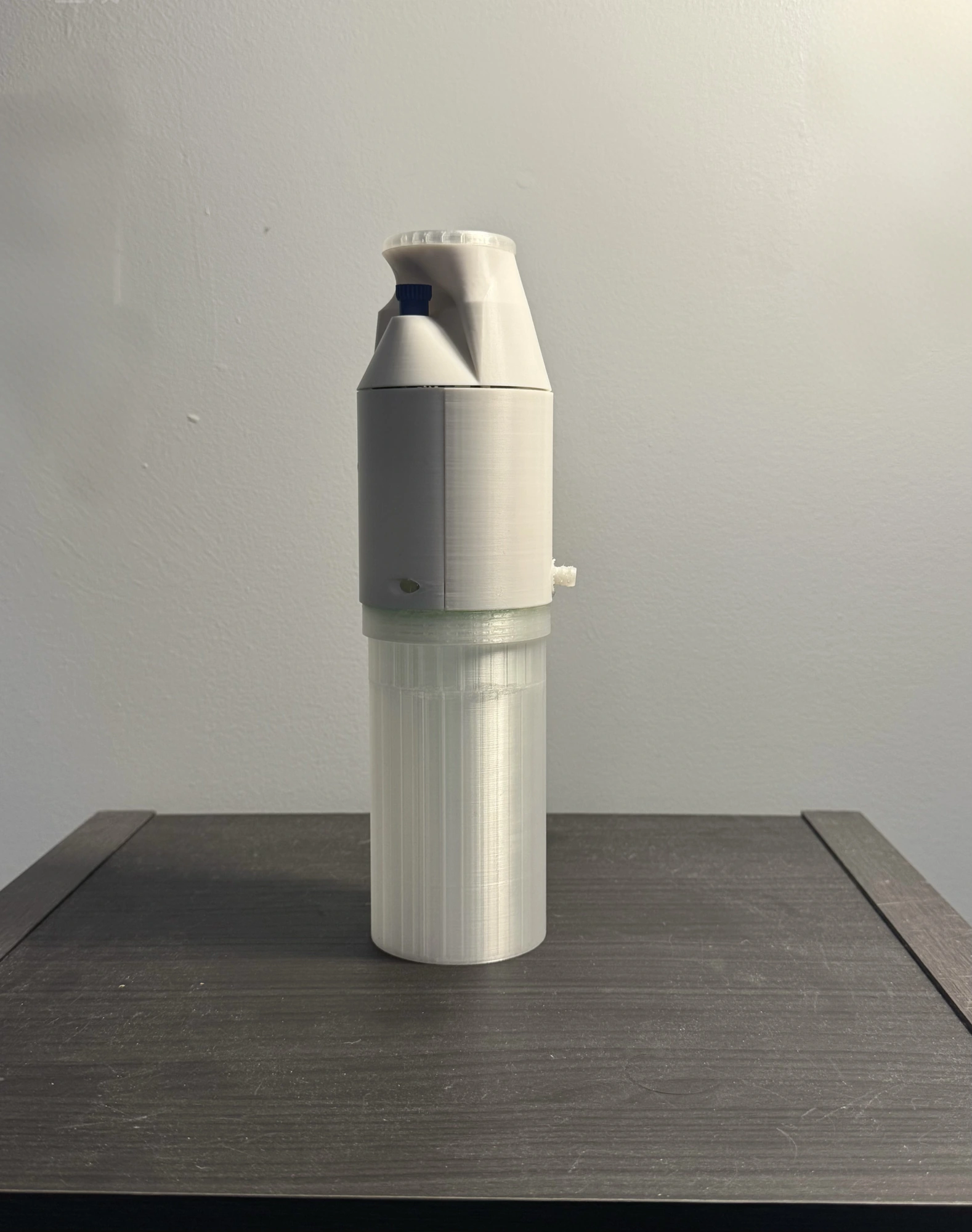
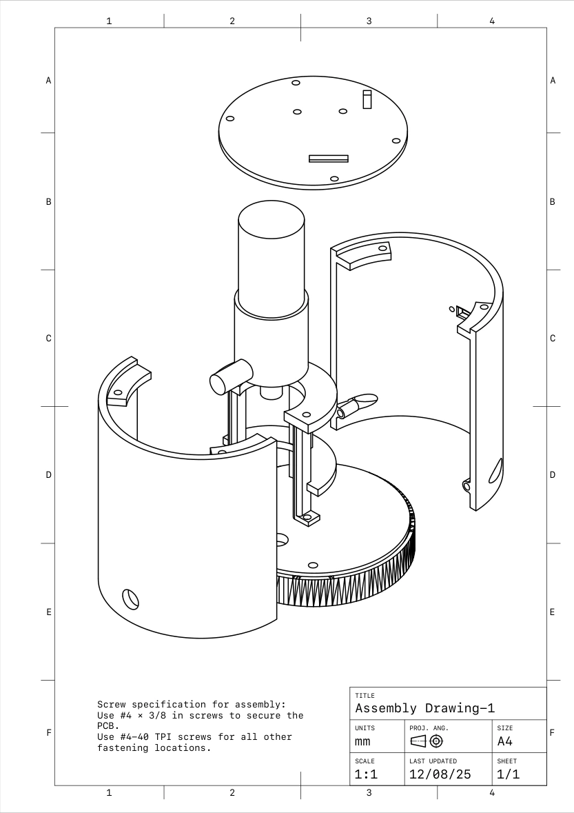
A dedicated pump cradle and upper platform establish component positions. The LCD holder, top shell and knob form a separate upper assembly with a defined installation sequence.
The split shell provides lateral access to install the pump, wiring and supports. Screw interfaces then close the housing around the assembly.
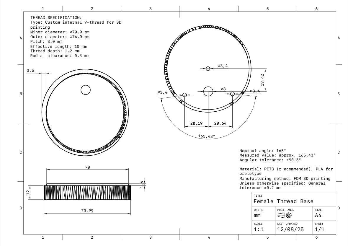
The cup’s threaded joint supports repeated removal while the screw-fastened shell keeps the internal assembly together. These interfaces serve different access needs.
A coarse V-thread gives the printer substantial features to form. Radial clearance accommodates variation between mating prints, while the engagement length distributes contact across several turns.
03 / Power architecture
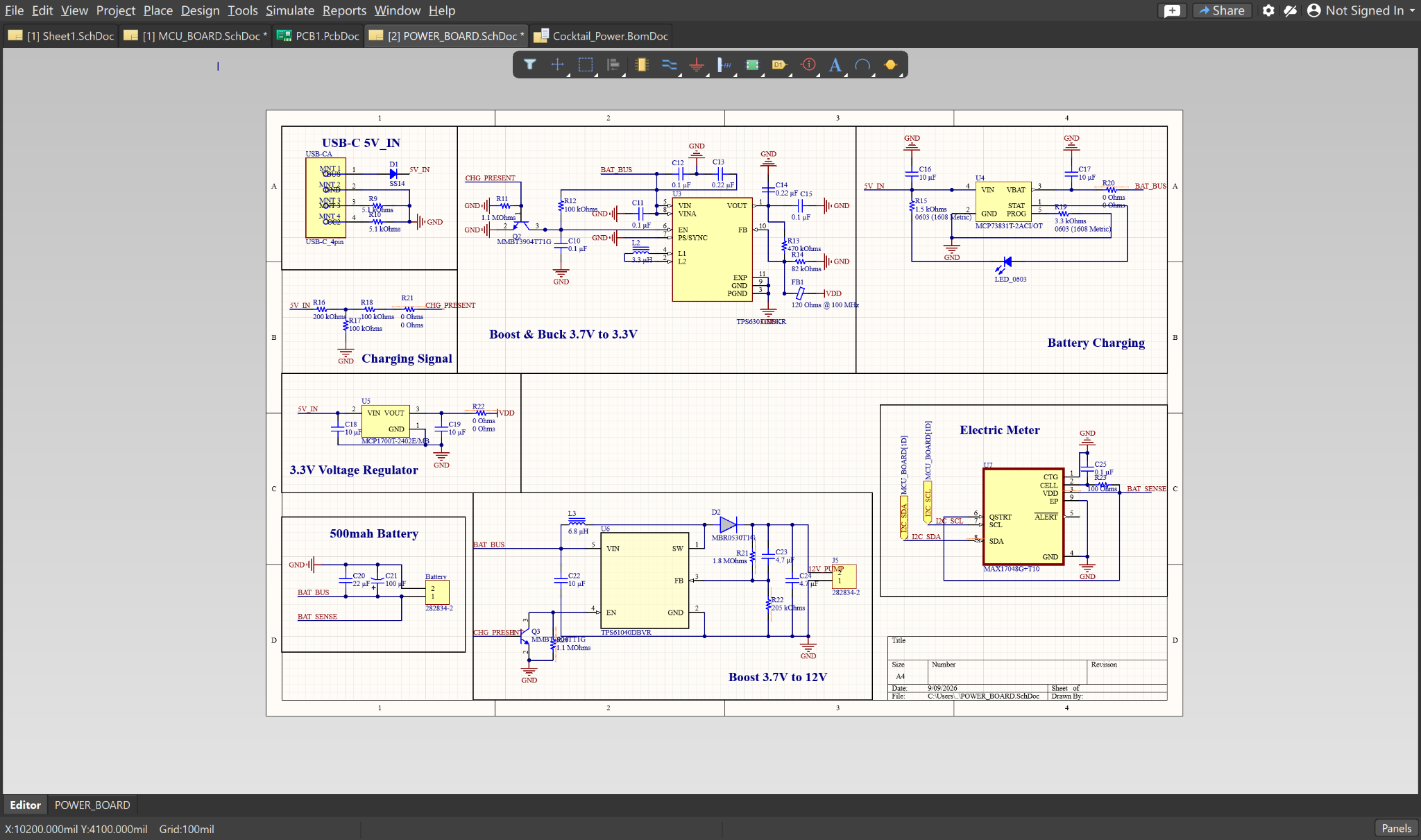
Rechargeable operation supports the handheld format. The cell’s 3.0–4.2 V range crosses the intended 3.3 V logic rail, requiring buck-boost regulation. A separate 12 V boost addresses the pump supply.
USB-C 5 V → Charger → 1S battery
MAX17048 battery monitor · I²C
USB-C feeds the MCP73831 charger. USB-presence detection pulls the battery-converter enable pins low, inhibiting the 12 V boost stage while USB is connected.
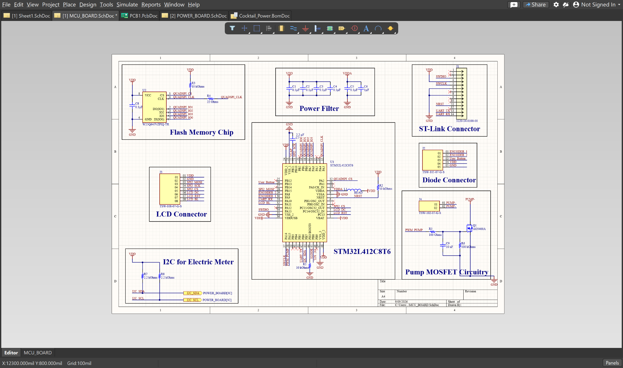
A MAX17048 reports battery state over I²C. The controller drives the pump through a MOSFET and connects the round LCD, rotary input and external flash.
04 / Electrical–mechanical integration
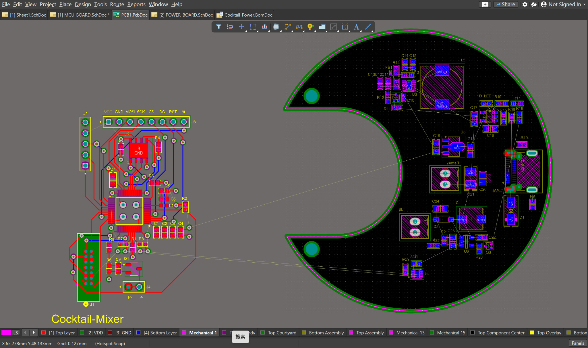
The C-shaped power-board outline allocates electronics around the mechanism. Central clearance, mounting positions and connector access tie its layout to the mechanical envelope.
Routing must keep converter switching loops compact, size the pump-current paths and preserve continuous returns within the enclosure’s clearance and mounting constraints.
05 / Prototype development
The printed prototype made the component fit, assembly sequence and removable cup tangible. Alongside the on-device interface, the pump bench setup demonstrated the liquid-transfer path.
The next integration step connects the recipe state, pump actuation and delivered volume. Dosing calibration and repeatability are the measurements needed to turn the guided workflow into a dependable product.
Project outcome
The work established the product architecture, schematics, PCB placement and partial routing, a printed assembly and subsystem demonstrations. Custom-board fabrication and full-system integration remained the next development stage.
MCU/control: Eddie. Firmware: Eddie and Stephanie.
Circuit sheets, mechanical drawings and full demonstrations.
Explore on GitHubUndergraduate thesis · 2024
Five-channel sensing for virtual-hand interaction.
Design intent
I designed and prototyped a physical controller that turns finger movement into a continuous response on a virtual hand. Contact-based sensing gives each movement a directly readable electrical signal, without camera input. My undergraduate project brings together the mechanical interface, STM32 acquisition, calibration, wireless communication and Unity visualization.
01 / Sensing through contact
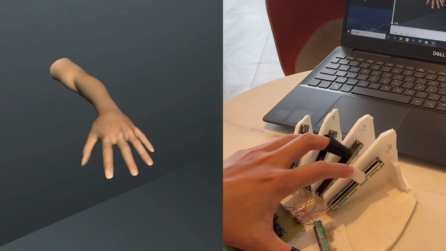
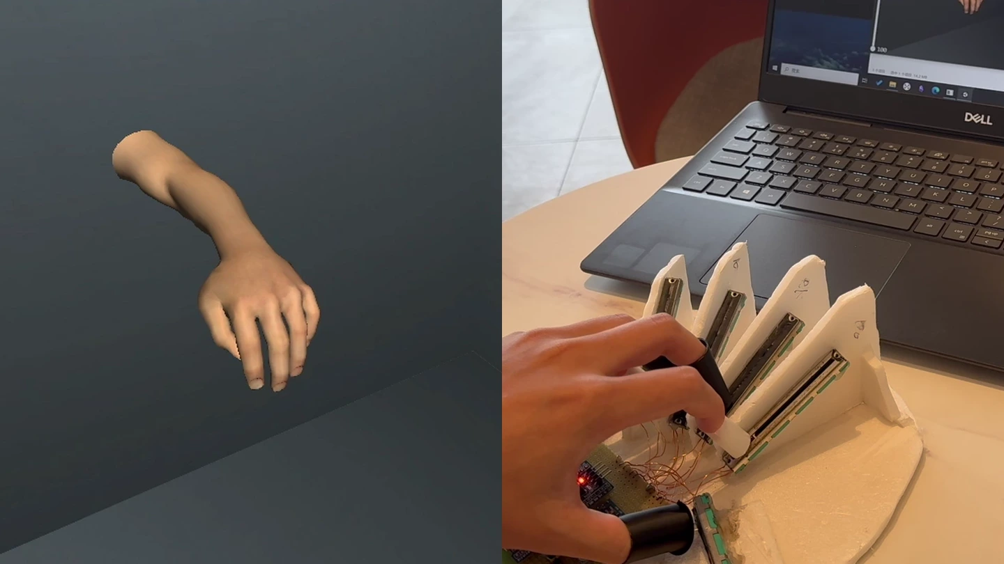
Each finger moves a linear potentiometer through a contact piece. Four inclined guides organize the main fingers; the thumb uses a separate direction of travel. The geometry connects how the hand moves with how the sensors measure it.
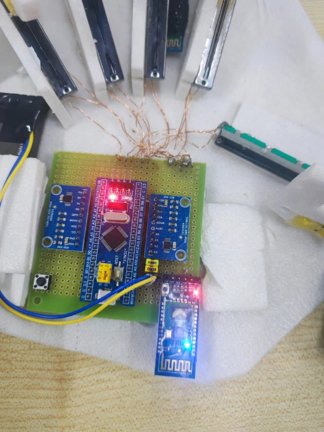
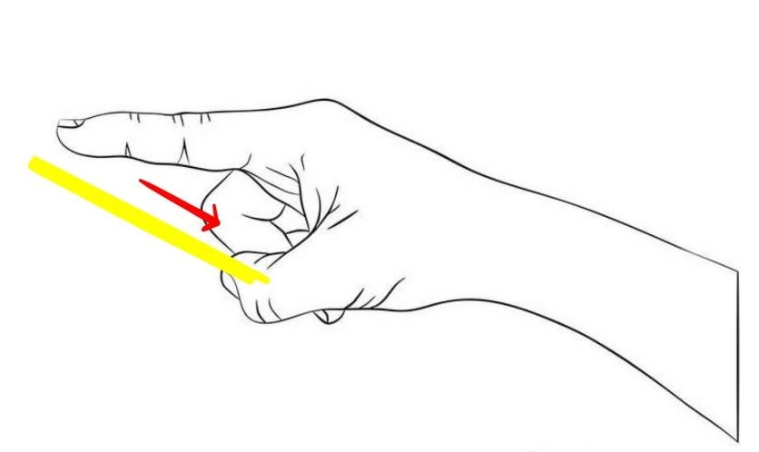
The guides constrain each contact piece to a measurable path. Finger length and contact position determine how much of the slider’s stroke the user can comfortably reach.
Five sensors produce five control values. This keeps acquisition and animation compact, with each value describing overall flexion rather than separate joint angles.
02 / Calibration
Different hands use different portions of the same slider. Endpoint capture establishes the usable stroke, while LED signals guide the user through setup. The thesis defines normalization relative to this travel range.
Sensor voltage → relative slider travel
Enter the calibration routine.
Move the calibration slider to minimum. The LED blinks slowly.
Move to the maximum position. Fast blinking confirms capture.
When blinking slows, check incoming states on the PC.
The saved v1 firmware shares one calibrated span across five channels. Independent endpoint pairs are the next step for adapting the mapping to each finger.
03 / Embedded-to-desktop integration
Two ADS1115 converters provide a 4 + 1 channel split over separate software I²C buses. The STM32 samples the inputs sequentially and transmits their latest stored states as a readable five-field frame.
5 sensor states
Software I²C
Bluetooth serial
115200 baud
USB receiver
Local TCP · 8086
Receive queue
Main-thread update
AT+020F1+056F2+060F3+090F4+050F5+EDA C# bridge owns the PC serial port and forwards bytes over local TCP. Unity receives data in the background, then drains queued samples on its main thread to update the hand.
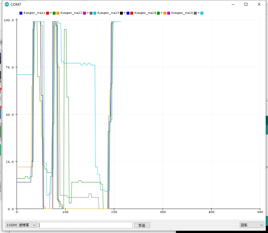
A hardware button switches between application frames and diagnostic output. The five-channel plot exposes sensor response directly, separating acquisition checks from animation behavior.
04 / Virtual-hand mapping
The Unity hand uses five flexion clips. C# divides each received percentage by 100 and places the corresponding clip at that normalized playback position, translating a control value into a visible pose.
Animation animation =
    fingerAnimation[index];
animation.Play();
animation["finger" + (index + 1)]
    .normalizedTime = value;
Invoke("stop", Time.deltaTime);Manual sliders drive the same finger controls without sensor input. This isolates the virtual-hand mapping before the wireless acquisition path is connected.
05 / Validation
The prototype can be inspected at three levels: the animation inputs, the captured signals and the assembled wireless interface. Each view exposes a different part of the same system.
Exercise each finger clip independently using the Unity sliders.
Inspect the five channel values as the fingers move.
Compare both sides of the interface and inspect timestamped records.
Outcome
The controller drives continuous pose changes in Unity. Five-channel waveform inspection and XLS export—timestamp, finger ID and value—make the captured states available beyond the animation.
Further development would focus on per-finger calibration, timer-driven acquisition and direct pose updates.
Virtual instrumentation · 2023
Part-relative measurement, contour matching and automated testing in LabVIEW.
The engineering problem
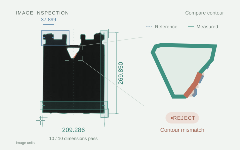
A connector can have the right dimensions and still contain a local shape defect.
I configured reference frames and measurement regions, integrated NI Vision caliper and contour tools, and built the LabVIEW state machine for image-folder inspection, result visualization and CSV logging.
01 / Registration
A fixed image region can miss the intended edge when a part moves. I used a measured coordinate system to position the dimensional ROIs relative to the connector. The central opening is checked through a separately configured contour region.
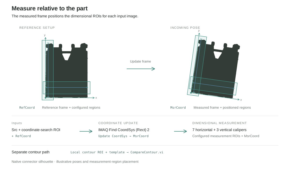
Separating localization from measurement keeps the search region and each caliper region independently adjustable. The image stays in its acquired coordinates; the dimensional tools receive the measured frame.
02 / Inspection logic
Seven horizontal and three vertical calipers measure detected edge-pair distances against a reference. The contour routine extracts the opening boundary, matches it to a learned template and evaluates corresponding-point distances. Both checks must pass.
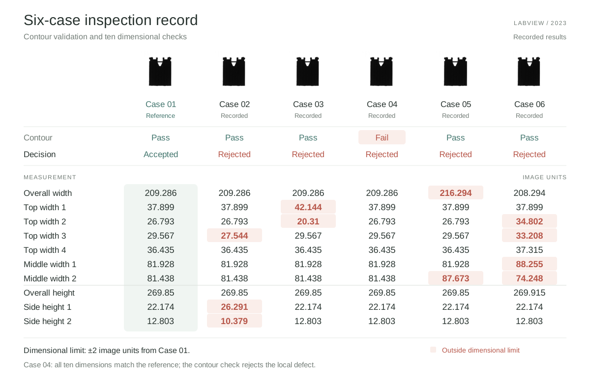
Contour match AND all ten dimensional checks within ±2 image units
03 / Application architecture
The state machine separates operator setup from the automatic inspection sequence. Shared configuration carries the reference frame, regions and dimensional limits between states, so each image is evaluated against the same settings.
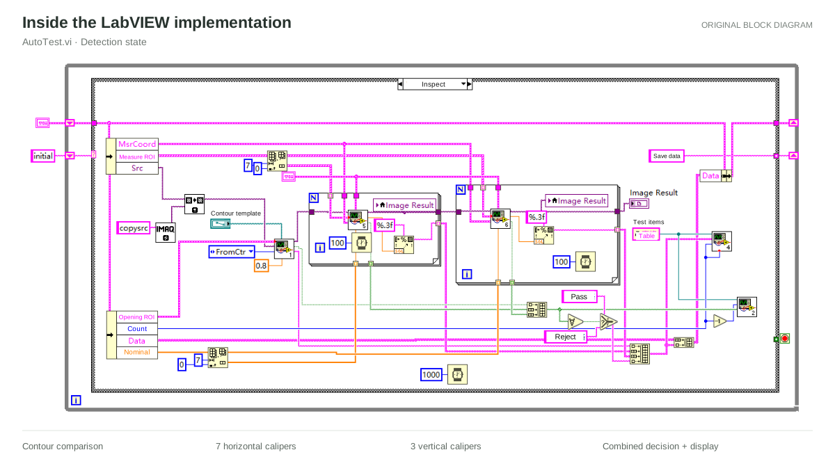
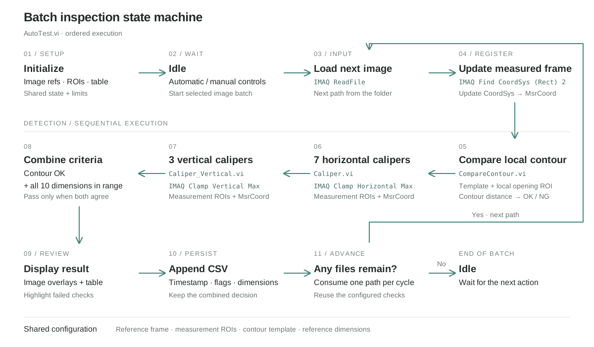
Separate horizontal-caliper, vertical-caliper and contour subVIs keep feature measurement distinct from the final decision.
Per-feature values and failed-cell highlights show why an image was rejected. CSV records retain the dimensions, contour flag, decision and timestamp.
Outcome
The application combines reusable setup, automatic image-folder inspection and per-feature CSV records. Across the six saved cases, it accepted the reference and rejected five altered parts.
Case 04 passed all ten dimensional checks but failed the contour check: selected dimensions alone cannot capture every local shape defect.
Practical design and technical support for a ranch owner.
A pro bono website upgrade for Jackson Ranch in Texas, carried out through Flynn Studio.
The design brings the herd, the ranch’s story, and visiting information into a clearer experience for people discovering the ranch online.
The visit flow is designed around a request followed by personal confirmation from the owner. It keeps the experience useful for visitors and manageable for the ranch.
The case study will follow the design decisions and final handoff as the project develops.